"Toom-3 is asymptotically O(N^1.465), the exponent being log(5)/log(3), representing 5 recursive multiplies of 1/3 the original size each. This is an improvement over Karatsuba at O(N^1.585), though Toom does more work in the evaluation and interpolation and so it only realizes its advantage above a certain size."
Reading http://gmplib.org/manual/Multiplication-Algorithms.html, it appears that GMP implements: Karatsuba, Toom-3, Toom-4, Toom-6.5, Toom-8.5, FFT -based multiplication methods, which I interpret to mean that Toom-Cook is useful for ranges between where Karatsuba and FFT are most useful.
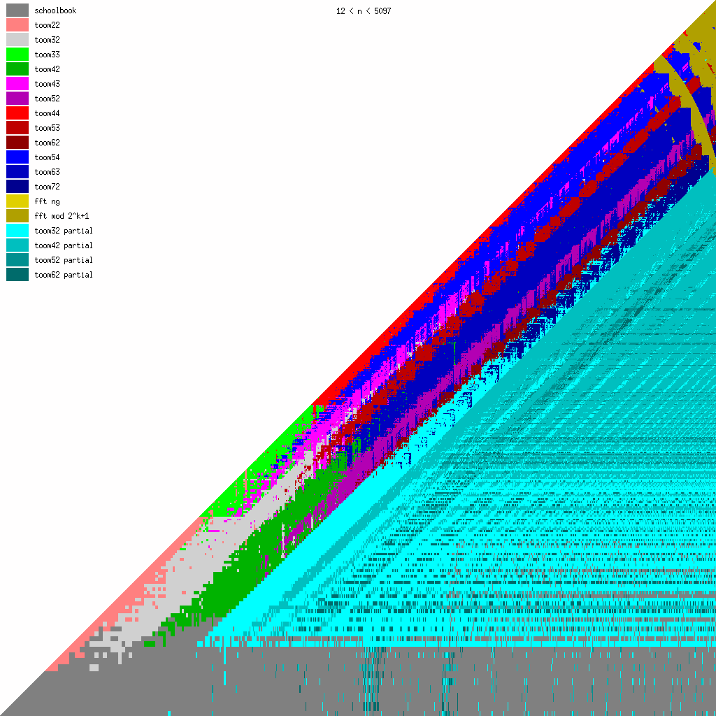
http://gmplib.org/devel/log.i7.1024.png
More context and explanation can be found at: http://gmplib.org/devel/
Short summary: Toom-Cook is nice because you have many parameters to play with.
What I like about it beyond the comprehensive coverage is that it explains the mathematical structure that underlies each of the algorithms. Unfortunately for HN readers, the paper's intended audience is mathematicians, but with a bit of background in algebra you might still be able to glean some useful insights.
As an example, I'll try to describe the Karatsuba trick.
We want to multiply two linear polynomials p = a + bx and q = c + dx. That is, we want to calculate the coefficients e, f, g in (a + bx)(c + dx) = e + fx + gx^2 in terms of a, b, c, d. The standard algorithm is e = ac, f = ad + bc, g = bd. This has 4 multiplications and 1 addition.
Here's the Karatsuba trick as usually presented. The word 'trick' is apt because this makes it seem like pulling a rabbit from a magician's hat. Let u = (a+b)(c+d) = ac + ad + bc + bd. Then f = u - ac - bd = u - e - g. Thus Karatsuba's trick calculates u = (a+b)(c+d), e = ac, g = bd, f = u-e-g. This has 3 multiplications and 4 additions. We've saved 1 multiplication at the expense of 3 extra additions.
If we now apply Karatsuba's trick recursively in divide-and-conquer fashion to the left and right halves of higher-degree polynomials, we get an algorithm that is faster than the standard algorithm even if we assume that scalar additions and multiplications have the same cost. The standard algorithm has cost O(n^2), where n is the degree of the polynomials, and Karatsuba's algorithm has cost O(n^(lg 3)), which is around O(n^1.6).
So what's the structure underlying Karatsuba's trick? Well, you might have noticed that u is p q evaluated at x = 1. You can evaluate a product of polynomials without multiplying them out first because evaluation is a homomorphism, so u = (p q)(1) = p(1) q(1).
Evaluation is a lossy (non-injective) mapping, so we will have to evaluate their product at three different points (since the product is quadratic and hence has three coefficients) to recover the original product uniquely. We've already evaluated at x = 1. Two other obvious candidate points for cheap evaluation are x = 0 and x = infinity. Evaluating at x = 0 just gives the constant term, so (p q)(0) = a c. Evaluating at x = infinity (make the substitution w = 1/x, clear denominators and evaluate at w = 0) gives the highest-degree term, so (p q)(infinity) = b d.
Now that we've evaluated the product at three points, all we have to do is interpolate between them with the Lagrange formula to recover the product.
That's the conceptual, geometric derivation of Karatsuba's trick.
This evaluate-and-interpolate approach is also what underlies FFT-based multiplication algorithms. The n-point FFT efficiently evaluates a polynomial at the nth roots of unity, which are the vertices of the regular n-gon on the unit circle in the complex plane. The inverse FFT efficiently interpolates an (n-1)-degree polynomial from its values at the nth roots of unity. The usual way of looking at FFT-based multiplication is via the convolution theorem (polynomial multiplication is convolution of the coefficient sequences). That may be more direct, but I like the unifying character of the evaluate-and-interpolate perspective.
Rather than use just evaluation, you can apply more general homomorphisms. That's how you get Toom's trick. If you've taken algebra, you'll recall that evaluation at a point t is just the quotient homomorphism for the maximal ideal (x - t).
If you find this intriguing, I suggest you study djb's paper.
Stratssen's algorithm, for multiplying matrices, uses a similar "trick". Naive matrix multiplication uses 8 steps for a (2x2) * (2x2), or n^3 multiplications. Stratssen's lowers this to 7 multiplications, and instead uses extra additions, thus achieving O(N^~2.807).
Edit: I've asked djb and we'll see if he responds.
The multimodular version is likewise pretty useless in practice.